Projection

The swiftsimio.visualisation.projection sub-module provides an interface to render SWIFT data projected to a grid. This takes your 3D data and projects it down to 2D, such that if you request masses to be smoothed then these functions return a surface density.

This effectively solves the equation:

\(\tilde{A}_i = \sum_j A_j W_{ij, 2D}\)

with \(\tilde{A}_i\) the smoothed quantity in pixel \(i\), and \(j\) all particles in the simulation, with \(W\) the 2D kernel. Here we use the Wendland-C2 kernel.

The primary function here is swiftsimio.visualisation.projection.project_gas(), which allows you to create a gas projection of any field. See the example below.

Example

from swiftsimio import load
from swiftsimio.visualisation.projection import project_gas

data = load("cosmo_volume_example.hdf5")

# This creates a grid that has units msun / Mpc^2, and can be transformed like
# any other unyt quantity
mass_map = project_gas(
    data,
    resolution=1024,
    project="masses",
    parallel=True,
    periodic=True,
)

# Let's say we wish to save it as msun / kpc^2,
from unyt import msun, kpc
mass_map.convert_to_units(msun / kpc**2)

from matplotlib.pyplot import imsave
from matplotlib.colors import LogNorm

# Normalize and save
imsave("gas_surface_dens_map.png", LogNorm()(mass_map.value), cmap="viridis")

This basic demonstration creates a mass surface density map.

To create, for example, a projected temperature map, we need to remove the surface density dependence (i.e. project_gas() returns a surface temperature in units of K / kpc^2 and we just want K) by dividing out by this:

from swiftsimio import load
from swiftsimio.visualisation.projection import project_gas

data = load("cosmo_volume_example.hdf5")

# First create a mass-weighted temperature dataset
data.gas.mass_weighted_temps = data.gas.masses * data.gas.temperatures

# Map in msun / mpc^2
mass_map = project_gas(
    data,
    resolution=1024,
    project="masses",
    parallel=True,
    periodic=True,
)
# Map in msun * K / mpc^2
mass_weighted_temp_map = project_gas(
    data,
    resolution=1024,
    project="mass_weighted_temps",
    parallel=True,
    periodic=True,
)

temp_map = mass_weighted_temp_map / mass_map

from unyt import K
temp_map.convert_to_units(K)

from matplotlib.pyplot import imsave
from matplotlib.colors import LogNorm

# Normalize and save
imsave("temp_map.png", LogNorm()(temp_map.value), cmap="twilight")

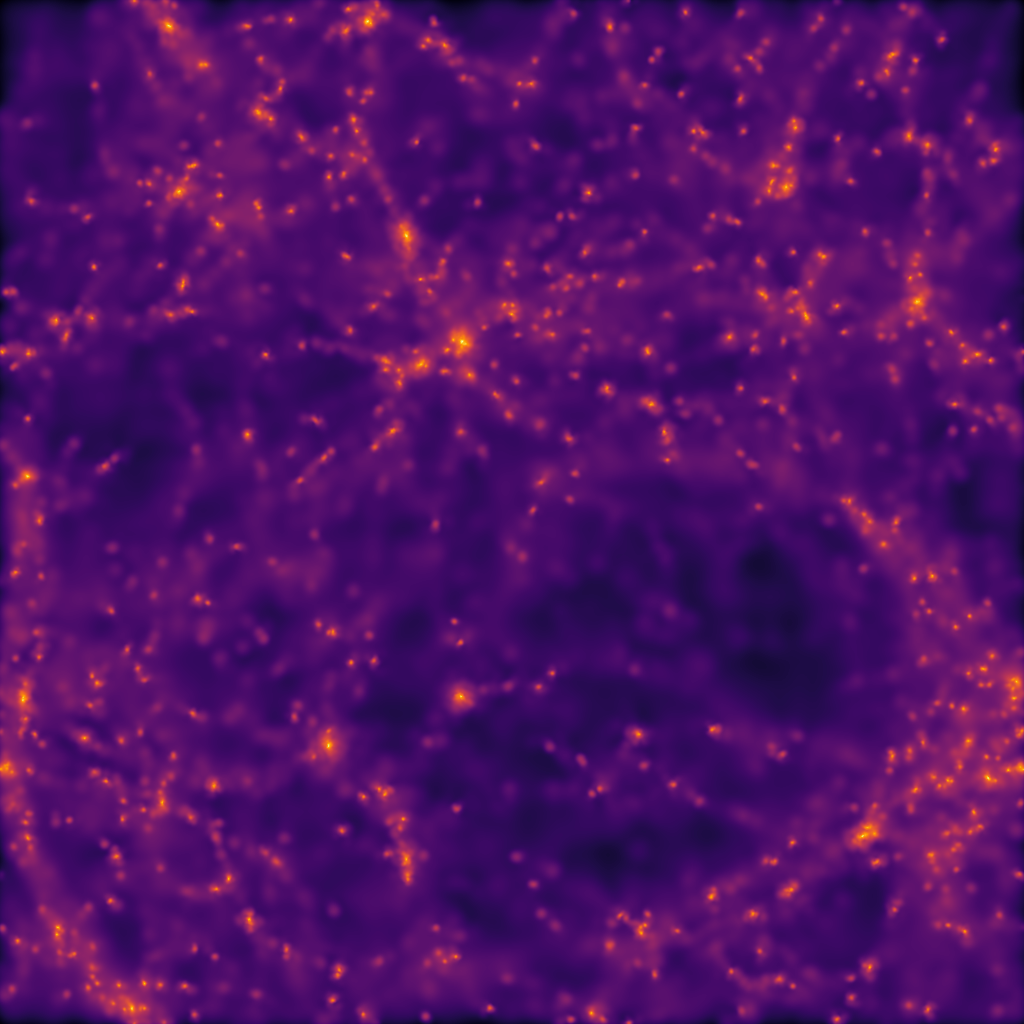
The output from this example, when used with the example data provided in the loading data section should look something like:

Backends

In certain cases, rather than just using this facility for visualisation, you will wish that the values that are returned to be as well converged as possible. For this, we provide several different backends. These are passed as backend="str" to all of the projection visualisation functions, and are available in the module swiftsimio.visualisation.projection.projection_backends. The available backends are as follows:

fast: The default backend - this is extremely fast, and provides very basic smoothing, with a return type of single precision floating point numbers.
histogram: This backend provides zero smoothing, and acts in a similar way to the np.hist2d function but with the same arguments as scatter.
reference: The same backend as fast but with two distinguishing features; all calculations are performed in double precision, and it will return early with a warning message if there are not enough pixels to fully resolve each kernel. Regular users should not use this mode.
renormalised: The same as fast, but each kernel is evaluated twice and renormalised to ensure mass conservation within floating point precision. Returns single precision arrays.
subsampled: This is the recommended mode for users who wish to have converged results even at low resolution. Each kernel is evaluated at least 32 times, with overlaps between pixels considered for every single particle. Returns in double precision.
subsampled_extreme: The same as subsampled, but provides 64 kernel evaluations.
gpu: The same as fast but uses CUDA for faster computation on supported GPUs. The parallel implementation is the same function as the non-parallel.

Example:

from swiftsimio import load
from swiftsimio.visualisation.projection import project_gas

data = load("cosmo_volume_example.hdf5")

subsampled_array = project_gas(
   data,
   resolution=1024,
   project="entropies",
   parallel=True,
   backend="subsampled",
   periodic=True,
)

This will likely look very similar to the image that you make with the default backend="fast", but will have a well-converged distribution at any resolution level.

Periodic boundaries

Cosmological simulations and many other simulations use periodic boundary conditions. This has implications for the particles at the edge of the simulation box: they can contribute to pixels on multiple sides of the image. If this effect is not taken into account, then the pixels close to the edge will have values that are too low because of missing contributions.

All visualisation functions by default assume a periodic box. Rather than simply projecting each individual particle once, four additional periodic copies of each particle are also projected. Most copies will project outside the valid pixel range, but the copies that do not ensure that pixels close to the edge receive all necessary contributions. Thanks to Numba optimisations, the overhead of these additional copies is relatively small.

There are some caveats with this approach. If you try to visualise a subset of the particles in the box (e.g. using a mask), then only periodic copies of particles in this subset will be used. If the subset does not include particles on the other side of the periodic boundary, then these will still be missing from the projection. The same is true if you visualise a region of the box. The periodic boundary wrapping is also not compatible with rotations (see below) and should therefore not be used together with a rotation.

Rotations

Sometimes you will need to visualise a galaxy from a different perspective. The swiftsimio.visualisation.rotation sub-module provides routines to generate rotation matrices corresponding to vectors, which can then be provided to the rotation_matrix argument of project_gas() (and project_gas_pixel_grid()). You will also need to supply the rotation_center argument, as the rotation takes place around this given point. The example code below loads a snapshot, and a halo catalogue, and creates an edge-on and face-on projection using the integration in velociraptor. More information on possible integrations with this library is shown in the velociraptor section.

from swiftsimio import load, mask
from velociraptor import load as load_catalogue
from swiftsimio.visualisation.rotation import rotation_matrix_from_vector
from swiftsimio.visualisation.projection import project_gas_pixel_grid

import unyt
import numpy as np
import matplotlib.pyplot as plt
from matplotlib.colors import LogNorm

# Radius around which to load data, we will visualise half of this
size = 1000 * unyt.kpc

snapshot_filename = "cosmo_volume_example.hdf5"
catalogue_filename = "cosmo_volume_example.properties"

catalogue = load_catalogue(catalogue_filename)

# Which halo should we visualise?
halo = 0

x = catalogue.positions.xcmbp[halo]
y = catalogue.positions.ycmbp[halo]
z = catalogue.positions.zcmbp[halo]

lx = catalogue.angular_momentum.lx[halo]
ly = catalogue.angular_momentum.ly[halo]
lz = catalogue.angular_momentum.lz[halo]

# The angular momentum vector will point perpendicular to the galaxy disk.
# If your simulation contains stars, use lx_star
angular_momentum_vector = np.array([lx.value, ly.value, lz.value])
angular_momentum_vector /= np.linalg.norm(angular_momentum_vector)

face_on_rotation_matrix = rotation_matrix_from_vector(
   angular_momentum_vector
)
edge_on_rotation_matrix = rotation_matrix_from_vector(
   angular_momentum_vector,
   axis="y"
)

region = [
   [x - size, x + size],
   [y - size, y + size],
   [z - size, z + size],
]

visualise_region = [
   x - 0.5 * size, x + 0.5 * size,
   y - 0.5 * size, y + 0.5 * size,
]

data_mask = mask(snapshot_filename)
data_mask.constrain_spatial(region)
data = load(snapshot_filename, mask=data_mask)

# Use project_gas_pixel_grid to generate projected images

common_arguments = dict(
    data=data,
    resolution=512,
    parallel=True,
    region=visualise_region,
    periodic=False, # disable periodic boundaries when using rotations
)

un_rotated = project_gas_pixel_grid(**common_arguments)

face_on = project_gas_pixel_grid(
   **common_arguments,
   rotation_center=unyt.unyt_array([x, y, z]),
   rotation_matrix=face_on_rotation_matrix,
)

edge_on = project_gas_pixel_grid(
   **common_arguments,
   rotation_center=unyt.unyt_array([x, y, z]),
   rotation_matrix=edge_on_rotation_matrix,
)

Using this with the provided example data will just show blobs due to its low resolution nature. Using one of the EAGLE volumes (examples/EAGLE_ICs) will produce much nicer galaxies, but that data is too large to provide as an example in this tutorial.

You can also provide an extra two values, the z min and max, as part of the region parameter. This may have some slight performance impact, so it is generally advised that you do this on sub-loaded volumes only.

Other particle types

Other particle types are able to be visualised through the use of the swiftsimio.visualisation.projection.project_pixel_grid() function. This does not attach correct symbolic units, so you will have to work those out yourself, but it does perform the smoothing. We aim to introduce the feature of correctly applied units to these projections soon.

To use this feature for particle types that do not have smoothing lengths, you will need to generate them, as in the example below where we create a mass density map for dark matter. We provide a utility to do this through swiftsimio.visualisation.smoothing_length_generation.generate_smoothing_lengths().

from swiftsimio import load
from swiftsimio.visualisation.projection import project_pixel_grid
from swiftsimio.visualisation.smoothing_length_generation import generate_smoothing_lengths

data = load("cosmo_volume_example.hdf5")

# Generate smoothing lengths for the dark matter
data.dark_matter.smoothing_length = generate_smoothing_lengths(
    data.dark_matter.coordinates,
    data.metadata.boxsize,
    kernel_gamma=1.8,
    neighbours=57,
    speedup_fac=2,
    dimension=3,
)

# Project the dark matter mass
dm_mass = project_pixel_grid(
    # Note here that we pass in the dark matter dataset not the whole
    # data object, to specify what particle type we wish to visualise
    data=data.dark_matter,
    boxsize=data.metadata.boxsize,
    resolution=1024,
    project="masses",
    parallel=True,
    region=None,
    periodic=True,
)

from matplotlib.pyplot import imsave
from matplotlib.colors import LogNorm

# Everyone knows that dark matter is purple
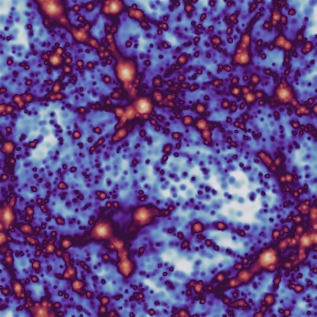
imsave("dm_mass_map.png", LogNorm()(dm_mass), cmap="inferno")

The output from this example, when used with the example data provided in the loading data section should look something like:

Lower-level API

The lower-level API for projections allows for any general positions, smoothing lengths, and smoothed quantities, to generate a pixel grid that represents the smoothed version of the data.

This API is available through swiftsimio.visualisation.projection.scatter() and swiftsimio.visualisation.projection.scatter_parallel() for the parallel version. The parallel version uses significantly more memory as it allocates a thread-local image array for each thread, summing them in the end. Here we will only describe the scatter variant, but they behave in the exact same way.

By default this uses the “fast” backend. To use the others, you can select them manually from the module, or by using the backends and backends_parallel dictionaries in swiftsimio.visualisation.projection.

To use this function, you will need:

x-positions of all of your particles, x.
y-positions of all of your particles, y.
A quantity which you wish to smooth for all particles, such as their mass, m.
Smoothing lengths for all particles, h.
The resolution you wish to make your square image at, res.

Optionally, you will also need: + the size of the simulation box in x and y, box_x and box_y.

The key here is that only particles in the domain [0, 1] in x, and [0, 1] in y will be visible in the image. You may have particles outside of this range; they will not crash the code, and may even contribute to the image if their smoothing lengths overlap with [0, 1]. You will need to re-scale your data such that it lives within this range. Then you may use the function as follows:

from swiftsimio.visualisation.projection import scatter

# Using the variable names from above
out = scatter(x=x, y=y, h=h, m=m, res=res)

out will be a 2D numpy grid of shape [res, res]. You will need to re-scale this back to your original dimensions to get it in the correct units, and do not forget that it now represents the smoothed quantity per surface area.

If the optional arguments box_x and box_y are provided, they should contain the simulation box size in the same re-scaled coordinates as x and y. The projection backend will then correctly apply periodic boundary wrapping. If box_x and box_y are not provided or set to 0, no periodic boundaries are applied.