Slices
The swiftsimio.visualisation.slice sub-module provides an interface
to render SWIFT data onto a slice. This takes your 3D data and finds the 3D
density at fixed z-position, slicing through the box.
The default "sph" backend effectively solves the equation:
\(\tilde{A}_i = \sum_j A_j W_{ij, 3D}\)
with \(\tilde{A}_i\) the smoothed quantity in pixel \(i\), and \(j\) all particles in the simulation, with \(W\) the 3D kernel. Here we use the Wendland-C2 kernel. Note that here we take the kernel at a fixed z-position.
There is also an alternative "nearest_neighbours" backend, which uses
nearest-neighbour interpolation to compute the densities at each pixel.
This backend is more suited for use with moving-mesh hydrodynamics schemes.
The primary functions here are
swiftsimio.visualisation.slice.slice_pixel_grid(), which allows you to
create a slice of any field for any particle type, and the convenience wrapper
swiftsimio.visualisation.slice.slice_gas() for gas particles. See the
examples below.
Example
from swiftsimio import load
from swiftsimio.visualisation.slice import slice_gas

data = load("cosmo_volume_example.hdf5")

# This creates a grid that has units msun / Mpc^3, and can be transformed like
# any other unyt quantity. The position of the slice along the z axis is
# provided in the z_slice argument.
mass_map = slice_gas(
    data,
    z_slice=0.5 * data.metadata.boxsize[2],
    resolution=1024,
    project="masses",
    parallel=True,
    periodic=True,
)

# Let's say we wish to save it as g / cm^2,
from unyt import g, cm
mass_map.convert_to_units(g / cm**3)

from matplotlib.pyplot import imsave
from matplotlib.colors import LogNorm

# Normalize and save
imsave("gas_slice_map.png", LogNorm()(mass_map.value), cmap="viridis")
This basic demonstration creates a mass density map.
To create, for example, a projected temperature map, we need to remove the
density dependence (i.e. slice_gas()
returns a volumetric temperature in units of K / kpc^3 and we just want K)
by dividing out by this:
from swiftsimio import load
from swiftsimio.visualisation.slice import slice_gas
data = load("cosmo_volume_example.hdf5")
# First create a mass-weighted temperature dataset
data.gas.mass_weighted_temps = data.gas.masses * data.gas.temperatures
# Map in msun / mpc^3
mass_map = slice_gas(
data,
z_slice=0.5 * data.metadata.boxsize[2],
resolution=1024,
project="masses",
parallel=True,
periodic=True,
)
# Map in msun * K / mpc^3
mass_weighted_temp_map = slice_gas(
data,
z_slice=0.5 * data.metadata.boxsize[2],
resolution=1024,
project="mass_weighted_temps",
parallel=True,
periodic=True,
)
temp_map = mass_weighted_temp_map / mass_map
from unyt import K
temp_map.convert_to_units(K)
from matplotlib.pyplot import imsave
from matplotlib.colors import LogNorm
# Normalize and save
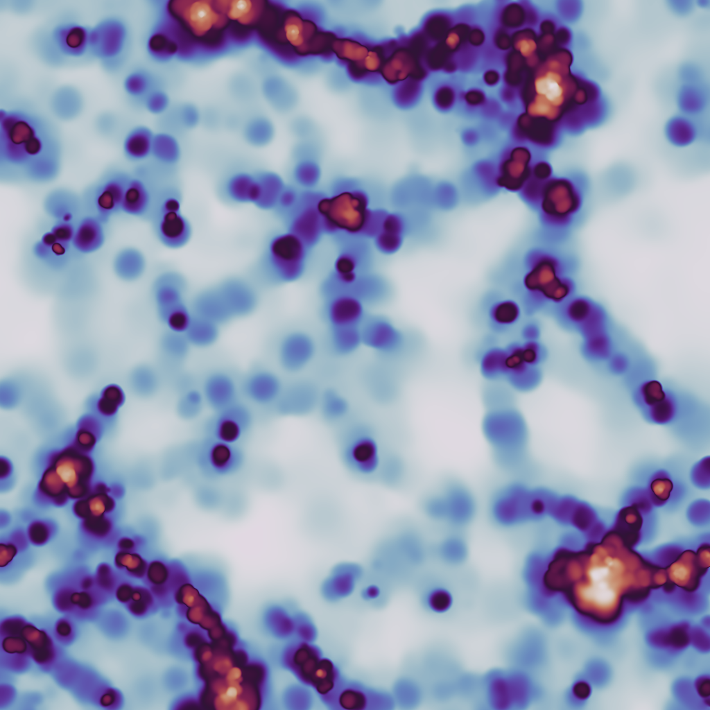
imsave("temp_map.png", LogNorm()(temp_map.value), cmap="twilight")
The output from this example, when used with the example data provided in the loading data section should look something like:
Periodic boundaries
Cosmological simulations and many other simulations use periodic boundary conditions. This has implications for the particles at the edge of the simulation box: they can contribute to pixels on multiple sides of the image. If this effect is not taken into account, then the pixels close to the edge will have values that are too low because of missing contributions.
All visualisation functions by default assume a periodic box. Rather than
simply summing each individual particle once, eight additional periodic copies
of each particle are also accounted for. Most copies will contribute outside the
valid pixel range, but the copies that do not ensure that pixels close to the
edge receive all necessary contributions. Thanks to numba optimisations, the
overhead of these additional copies is relatively small.
There are some caveats with this approach. If you try to visualise a subset of the particles in the box (e.g. using a mask), then only periodic copies of particles in this subset will be used. If the subset does not include particles on the other side of the periodic boundary, then these will still be missing from the slice. The same is true if you visualise a region of the box. The periodic boundary wrapping is also not compatible with rotations (see below) and should therefore not be used together with a rotation.
Rotations
Rotations of the box prior to slicing are provided in a similar fashion to the
swiftsimio.visualisation.projection sub-module, by using the
swiftsimio.visualisation.rotation sub-module. To rotate the perspective
prior to slicing a rotation_center argument in
slice_gas() needs
to be provided, specifying the point around which the rotation takes place.
The angle of rotation is specified with a matrix, supplied by rotation_matrix
in slice_gas(). The rotation matrix may
be computed with
rotation_matrix_from_vector(). This will
result in the perspective being rotated to be along the provided vector. This
approach to rotations applied to the above example is shown below.
from swiftsimio import load
from swiftsimio.visualisation.slice import slice_gas
from swiftsimio.visualisation.rotation import rotation_matrix_from_vector

data = load("cosmo_volume_example.hdf5")

# First create a mass-weighted temperature dataset
data.gas.mass_weighted_temps = data.gas.masses * data.gas.temperatures

# Specify the rotation parameters
center = 0.5 * data.metadata.boxsize
rotate_vec = [0.5, 0.5, 1]
matrix = rotation_matrix_from_vector(rotate_vec, axis='z')

# Map in msun / mpc^3
# If a rotation center is provided, z_slice is taken relative to this
# center, resulting in a slice perpendicular to the rotated z axis
mass_map = slice_gas(
    data,
    z_slice=0. * data.metadata.boxsize[2],
    resolution=1024,
    project="masses",
    rotation_matrix=matrix,
    rotation_center=center,
    parallel=True,
    periodic=False,  # disable periodic boundaries when using rotations
)

# Map in msun * K / mpc^3
mass_weighted_temp_map = slice_gas(
    data,
    z_slice=0. * data.metadata.boxsize[2],
    resolution=1024,
    project="mass_weighted_temps",
    rotation_matrix=matrix,
    rotation_center=center,
    parallel=True,
    periodic=False,
)

temp_map = mass_weighted_temp_map / mass_map

from unyt import K
temp_map.convert_to_units(K)

from matplotlib.pyplot import imsave
from matplotlib.colors import LogNorm

# Normalize and save
imsave("temp_map.png", LogNorm()(temp_map.value), cmap="twilight")
Masking
Sometimes you want to render only a subset of a snapshot’s data, for example
just particles belonging to a given friends-of-friends group.
To achieve this, you can provide a boolean mask to
slice_pixel_grid() or
slice_gas() to render only the
particles which the mask specifies.
from swiftsimio import load, mask, cosmo_array
from swiftsimio.visualisation.slice import slice_gas

snapshot_filename = "cosmo_volume_example.hdf5"
catalog_filename = "fof_output_example.hdf5"

# Which halo are we looking at?
halo = 0

fof_catalog = load(catalog_filename)

fof_id = fof_catalog.fof_groups.group_ids[halo]
fof_radius = fof_catalog.fof_groups.radii[halo]
fof_centre = fof_catalog.fof_groups.centres[halo]

# Add some buffer space around the edges
fof_radius *= 1.1

# Define a region around the fof group
region = cosmo_array(
    [
        [fof_centre[0] - fof_radius, fof_centre[0] + fof_radius],
        [fof_centre[1] - fof_radius, fof_centre[1] + fof_radius],
        [fof_centre[2] - fof_radius, fof_centre[2] + fof_radius],
    ],
    fof_centre.units,
    comoving=True,
    scale_factor=fof_catalog.metadata.a,
    scale_exponent=1,
)

# Only load data in our region of interest
data_mask = mask(snapshot_filename)
data_mask.constrain_spatial(region)

data = load(snapshot_filename, mask=data_mask)

halo_slice = slice_gas(
    data,
    z_slice=fof_centre[2],
    resolution=512,
    parallel=True,
    region=region.ravel(),
    periodic=True,
    mask=data.gas.fofgroup_id == fof_id, # Only render particles in the group
)
Other particle types
Other particle types can be sliced using
swiftsimio.visualisation.slice.slice_pixel_grid().
For particle types that do not have smoothing lengths (e.g. dark matter),
you will need to generate them first using
generate_smoothing_lengths().
from swiftsimio import load
from swiftsimio.visualisation.slice import slice_pixel_grid
from swiftsimio.visualisation.smoothing_length import generate_smoothing_lengths

data = load("cosmo_volume_example.hdf5")

# Generate smoothing lengths for the dark matter
data.dark_matter.smoothing_length = generate_smoothing_lengths(
    data.dark_matter.coordinates,
    data.metadata.boxsize,
    kernel_gamma=1.8,
    neighbours=57,
    speedup_fac=2,
    dimension=3,
)

# Slice the dark matter mass at the midplane
dm_mass_slice = slice_pixel_grid(
    # Pass the dark matter dataset, not the whole data object
    data=data.dark_matter,
    z_slice=0.5 * data.metadata.boxsize[2],
    resolution=1024,
    project="masses",
    parallel=True,
    periodic=True,
)

from matplotlib.pyplot import imsave
from matplotlib.colors import LogNorm

imsave("dm_mass_slice.png", LogNorm()(dm_mass_slice.value), cmap="inferno")
Lower-level API
The lower-level API for slices allows for any general positions, smoothing lengths, and smoothed quantities, to generate a pixel grid that represents the smoothed, sliced, version of the data.
This API is available through
swiftsimio.visualisation.slice_backends.backends and
swiftsimio.visualisation.slice_backends.backends_parallel for parallel
implementations. The parallel versions uses significantly more memory as they allocate
a thread-local image array for each thread, summing them in the end. Here we
will only describe the sph variant, but they behave in the exact same way.
To use this function, you will need:
x-positions of all of your particles,
x.y-positions of all of your particles,
y.z-positions of all of your particles,
z.Where in the range you wish to slice,
z_slice.A quantity which you wish to smooth for all particles, such as their mass,
m.Smoothing lengths for all particles,
h.The resolution you wish to make your square image at,
res.
Optionally, you will also need:
+ the size of the simulation box in x, y and z, box_x, box_y and box_z.
The key here is that only particles in the domain [0, 1] in x and y will be
visible in the image. You may have particles outside of this range; they will
not crash the code, and may even contribute to the image if their smoothing
lengths overlap with [0, 1]. You will need to re-scale your data such that it
lives within this range. Smoothing lengths and z coordinates need to be
re-scaled in the same way (using the same scaling factor), but z coordinates do
not need to lie in the domain [0, 1]. You should provide inputs as raw numpy arrays
(not cosmo_array or unyt_array).
Then you may use the function as follows:
from swiftsimio.visualisation.slice_backends import backends

slice_scatter = backends["sph"]
# Using the variable names from above
out = slice_scatter(x=x, y=y, z=z, h=h, m=m, z_slice=z_slice, res=res)
out will be a 2D numpy grid of shape [res, res]. You will need
to re-scale this back to your original dimensions to get it in the correct units,
and do not forget that it now represents the smoothed quantity per volume.
If the optional arguments box_x, box_y and box_z are provided, they
should contain the simulation box size in the same re-scaled coordinates as
x, y and z. The slicing function will then correctly apply
periodic boundary wrapping. If box_x, box_y and box_z are not
provided or set to 0, no periodic boundaries are applied.